\(\text{CauchyVariate}\)

You can use the \(\text{CauchyVariate}\) function to calculate one or more random variates in a Cauchy-Lorentz distribution.

You can use the \cauchyv backslash command to insert this function.

The following variants of this function are available:

• \(\text{real } \text{CauchyVariate} \left ( \text{<location>}, \text{<}\gamma\text{>} \right )\)

• \(\text{real matrix } \text{CauchyVariate} \left ( \text{<number rows>}, \text{<number columns>}, \text{<location>}, \text{<}\gamma\text{>} \right )\)

Where \(x\), \(location\), and \(\gamma\) are scalar values representing the value of interest, the location or offset, and the scale term respectively. Note that this function is defined over the range \(\gamma > 0\) and will generate a runtime error, return NaN or a matrix of NaN for all other values.

The four parameter version, which includes \(\text{<number rows>}\) and \(\text{<number columns>}\) fields, returns an real matrix returning random deviates. The two parameter version returns a single value.

This function calculates random variates using transformation method based on the definition of the Cauchy-Lorentz quantile function:

\[\text{CauchyVariate} \left ( l, \gamma \right ) = x _ 0 + \gamma \tan \left [ \pi \left ( p - \frac{1}{2} \right ) \right ]\]

where \(p\) is a random variate in a uniform distribution over the range \(0 < p < 1\), and \(x _ 0\) is the location term.

Figure 115 shows the basic use of the \(\text{CauchyVariate}\) function.

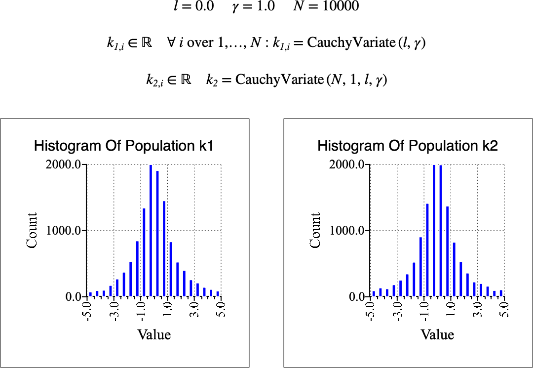
Figure 115 Example Use Of The CauchyVariate Function