\(\text{DCT}_3\)

Calculates the type 3 discrete cosine transform, of a matrix in one or two dimensions. This transform is the inverse of the type 2 discrete cosine transform.

You can use the \dct3 backslash command to insert this function.

The following variants of this function are available:

• \(\text{real matrix } \text{DCT}_3 \left ( \text{<matrix>} \right )\)

The \(\text{DCT}_3\) accepts boolean, integer, or real matrices and returns a real matrix containing the type 3 or inverse DCT. The input matrix can be a row matrix, column matrix or a 2 dimensional matrix. The returned matrix will have the same dimensions as the supplied input matrix.

This function calculates the DFT in one dimension using the relation:

\[\begin{split}C _ k = \begin{cases} \frac{1}{\sqrt{N}} & k = 1 \\ \frac{\sqrt{2}}{\sqrt{N}} & k \ne 1 \\ \end{cases}\end{split}\]

\[y _ n = \sum_{k=1}^N C _ k x_k \cos \frac{\left ( 2 n - 1 \right ) \pi \left ( k - 1 \right ) } {2N}\]

\[\forall n \in \left \lbrace 1 \ldots N \right \rbrace\]

The two dimensional DCT relies on the property of orthogonality. A DCT is first calculated independently on each row, creating a partially transformed matrix. A DCT is then calculated on each column of the partially transformed matrix.

Figure 123 shows the basic use of the \(\text{DFT}_3\) function.

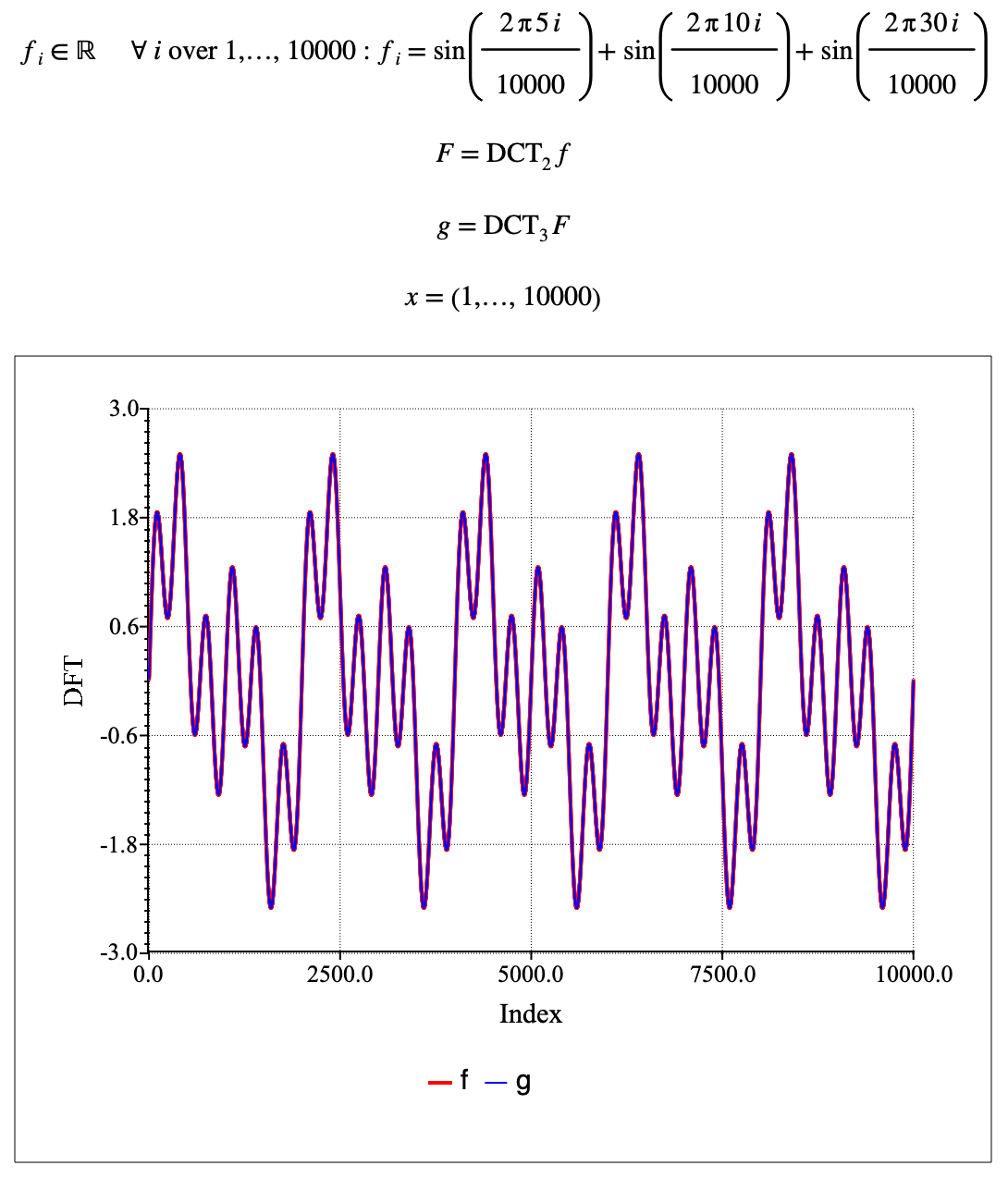
Figure 123 Example Use of The Type 3 DCT Function