\(\text{GammaPDF}\)
You can use the \(\text{GammaPDF}\) function to calculate the probability density function (PDF) of the gamma distribution.
You can use the \gammap backslash command to insert this function.
The following variants of this function are available:
\(\text{real } \text{GammaPDF} \left ( \text{<x>}, \text{<k>} \right )\)
\(\text{real } \text{GammaPDF} \left ( \text{<x>}, \text{<k>}, \text{<}\theta\text{>} \right )\)
Where \(x\), \(k\), and \(\theta\) are scalar values
representing the value of interest, the shape term, and the scale term
respectively. Note that this function is defined over the range
\(x \geq 0\), \(k > 0\), and \(\theta > 0\) and will generate an
error or return NaN for values for which the function is not defined.
The \(\theta\) term is optional. The value 1 will be used if the
\(\theta\) term is not provided.
The value is calculated directly using the relation:
The gamma distribution can be viewed as the sum of \(k\) identical and independent exponential distributions, each with rate \(\frac{1}{\theta}\). The exponential distribution is therefore the special case of the gamma distribution with \(k = 1\). Similarly, the gamma distribution is also equivalent to the Erlang distribution when \(k\) is an integer value.
The gamma distribution is identical to the chi-squared distribution with \(v\) degrees of freedom when \(k = \frac{1}{2} v\) and \(\theta = 2\).
Figure 144 shows the basic use of the \(\text{GammaPDF}\) function.
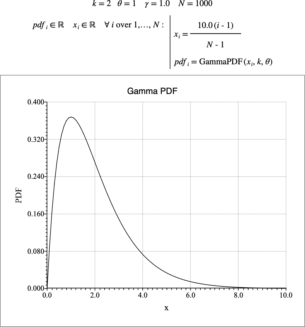
Figure 144 Example Use Of the GammaPDF Function