\(\text{GammaVariate}\)
You can use the \(\text{GammaVariate}\) function to calculate one or more random variates in a gamma distribution.
You can use the \gammav backslash command to insert this function.
The following variants of this function are available:
\(\text{real } \text{GammaVariate} \left ( \text{<k>} \right )\)
\(\text{real } \text{GammaVariate} \left ( \text{<k>}, \text{<}\theta\text{>} \right )\)
\(\text{real matrix } \text{GammaVariate} \left ( \text{<number rows>}, \text{<number columns>}, \text{<k>} \right )\)
\(\text{real matrix } \text{GammaVariate} \left ( \text{<number rows>}, \text{<number columns>}, \text{<k>}, \text{<}\theta\text{>} \right )\)
Where \(k\), and \(\theta\) are scalar values representing the shape
shape term and the scale term respectively. Note that these functions are
defined over the range \(k > 0\) and \(\theta > 0\) and will generate
an error or return NaN for values for which the function is not defined.
The three and four parameter versions, which includes \(\text{<number rows>}\) and \(\text{<number columns>}\) fields, returns an real matrix returning random deviates. The one and two parameter versions return a single value.
This function calculates random variates using the method described in [3].
The gamma distribution can be viewed as the sum of \(k\) identical and independent exponential distributions with rate \(\frac{1}{\theta}\). The exponential distribution is therefore the special case of the gamma distribution with \(k = 1\). Similarly, the gamma distribution is also equivalent to the Erlang distribution when \(k\) is an integer value.
The gamma distribution is identical to the chi-squared distribution with \(v\) degrees of freedom when \(k = \frac{1}{2} v\) and \(\theta = 2\).
Figure 146 shows the basic use of the \(\text{GammaVariate}\) function.
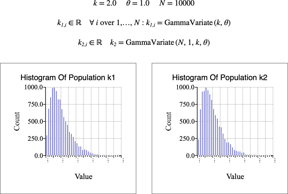
Figure 146 Example Use Of The GammaVariate Function