\(\text{InverseDFT}\)
Calculates the inverse discrete Fourier transform (DFT) of a matrix in one or two dimensions.
You can use the \idft backslash command to insert this function.
The following variants of this function are available:
\(\text{complex matrix } \text{InverseDFT} \left ( \text{<matrix>} \right )\)
The \(\text{InverseDFT}\) always returns a complex matrix independent of the type of the supplied input. Also note that the function assumes a cartesian representation of complex values rather than a polar representation. The returned matrix will have the same dimensions as the supplied input matrix.
This function calculates the inverse DFT in one dimension using the relation:
In two dimensions, this function calculates the DFT using the relation:
Figure 159 shows the basic use of the \(\text{InverseDFT}\) function.
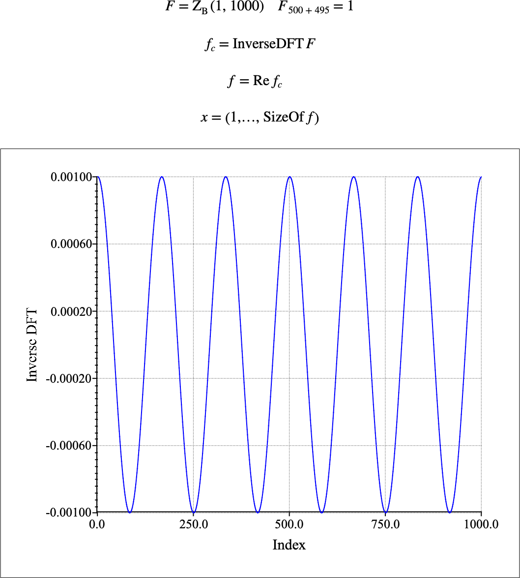
Figure 159 Example Use of The Inverse DFT Function