\(\text{NormalPDF}\)

You can use the \(\text{NormalPDF}\) function to calculate the probability density function (PDF) of the normal or Gaussian distribution.

You can use the \normalp backslash command to insert this function.

The following variants of this function are available:

• \(\text{real } \text{NormalPDF} \left ( \text{<x>} \right )\)

• \(\text{real } \text{NormalPDF} \left ( \text{<x>}, \text{<}\mu\text{>} \right )\)

• \(\text{real } \text{NormalPDF} \left ( \text{<x>}, \text{<}\mu\text{>}, \text{<}\sigma\text{>} \right )\)

The \(\text{x}\), \(\text{<}\mu\text{>}\), and \(\text{<}\sigma\text{>}\) are scalar values representing the value of interest, the mean value of the distribution, and the standard deviation respectively. The \(\text{<}\mu\text{>}\) and \(\text{<}\sigma\text{>}\) parameters are optional. If the \(\text{<}\mu\text{>}\) parameter is not included, a value of 0 is used. If the \(\text{<}\sigma\text{>}\) parameter is not included, a value of 1 is used. Note that the function is defined over the range \(\sigma > 0\) and will generate a run-time error or return NaN for values for which the function is not defined.

The returned value is calculated directly using the relation:

\[\text{NormalPDF} \left ( x, \mu, \sigma \right ) = \frac{1}{\sigma \sqrt{ 2 \pi }} e ^ { -\frac{1}{2} \left ( \frac{x - \mu}{\sigma} \right ) ^ 2 }\]

The normal distribution is one of the most widely used distribution as it represents the sum of a large number of random processes with fininte mean and variance. The resulting distribution from the sum will approach the normal distribution as the number of random processes approaches infinity. In practice, only a small number of random processes are needed to obtain a close approximation of the normal distribution.

Figure 181 shows the basic use of the \(\text{NormalPDF}\) function.

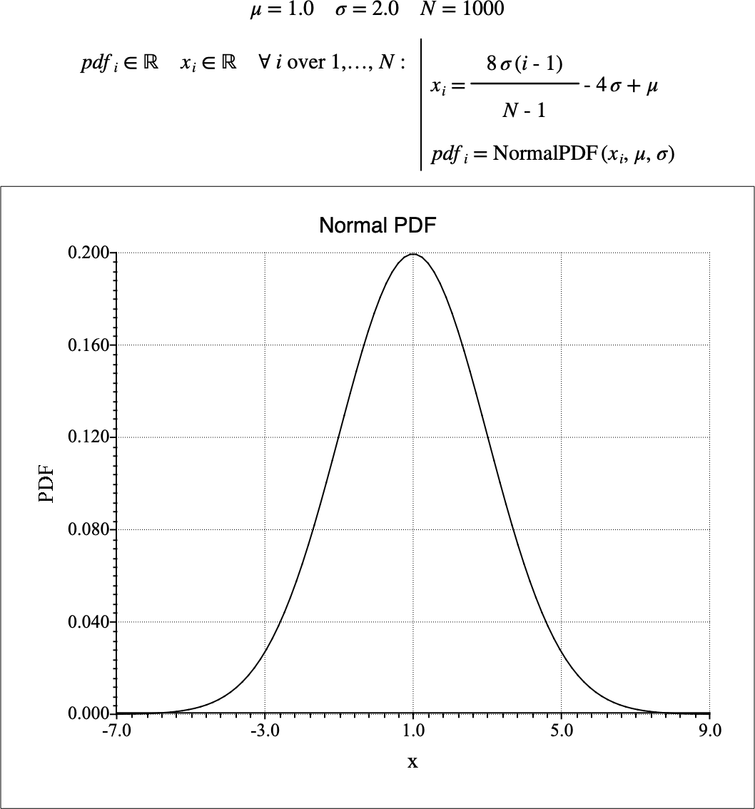
Figure 181 Example Use Of the NormalPDF Function