\(\text{PoissonVariate}\)
You can use the \(\text{PoissonVariate}\) function to calculate one or more random variates in a Poisson distribution.
You can use the \poissonv backslash command to insert this function.
The following variants of this function are available:
\(\text{integer } \text{PoissonVariate} \left ( \text{<}\lambda\text{>} \right )\)
\(\text{integer matrix } \text{PoissonVariate} \left ( \text{<number rows>}, \text{<number columns>}, \text{<}\lambda\text{>} \right )\)
Where \(\lambda\) is a scalar value representing the rate. The function is
defined over \(\lambda > 0\) and will generate a runtime error, return
NaN, or a matrix of NaN for values for which the function is not
defined.
The single parameter version of this function will return a single random variate in a Poisson distribution. The three parameter version will return a matrix of random variates.
Note that this function is defined over the range \(\gamma > 0\) and will
generate a runtime error, return NaN or a matrix of NaN for all other
values.
The three parameter version, which includes \(\text{<number rows>}\) and \(\text{<number columns>}\) fields, returns an real matrix returning random deviates. The two parameter version returns a single value.
This function calculate random variates using transformation method based on the definition of the Cauchy-Lorentz quantile function:
The \(\text{PoissonVariate}\) function uses Knuth’s algorithm [6] for cases where \(\lambda \leq 12\). For values greater than 12, the \(\text{PoissonVariate}\) uses a proprietary rejection method.
The Poisson distribution models the the number of events over a given time time period caused by a memoryless process and, in this respect, is closely related to the exponential distribution that models time between events assuming a memoryless process.
Figure 189 shows the basic use of the \(\text{PoissonVariate}\) function.
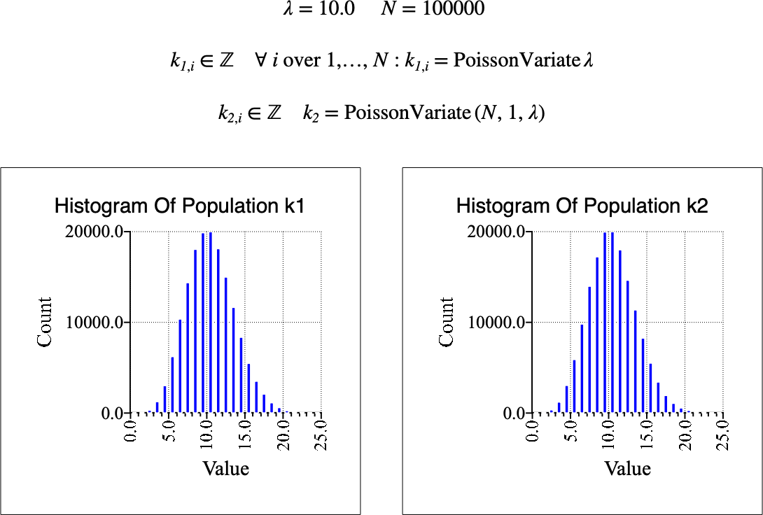
Figure 189 Example Use Of The PoissonVariate Function