\(\text{WeibullQuantile}\)

You can use the \(\text{WeibullQuantile}\) function to calculate the quantile function of the Weibull distribution. The quantile function is the inverse of the cumulative distribution function.

You can use the \weibullq backslash command to insert this function.

The following variants of this function are available:

• \(\text{real } \text{WeibullQuantile} \left ( \text{<p>}, \text{<k>}, \text{<}\lambda\text{>} \right )\)

• \(\text{real } \text{WeibullQuantile} \left ( \text{<p>}, \text{<k>}, \text{<}\lambda\text{>}, \text{<delay>} \right )\)

Where \(\text{<p>}\), \(\text{<k>}\), and \(\text{<}\lambda\text{>}\) are scalar values representing the cumulative probability, the shape term, and the scale term respectively. The \(\text{WeibullQuantile}\) function is defined over the range \(0 \leq p \leq 1\), \(k > 0\), and \(\lambda > 0\) and will generate an error or return NaN for values for which the function is not defined.

The \(\text{<delay>}\) term is optional. If not specified, a delay of 0 is used.

The value is calculated directly using the relation:

\[\text{WeibullQuantile} \left ( p, k, \lambda, delay \right ) = delay + \lambda \left [ - \ln \left ( 1 - p \right ) \right ] ^ \frac{1}{k}\]

Figure 221 shows the basic use of the \(\text{WeibullQuantile}\) function.

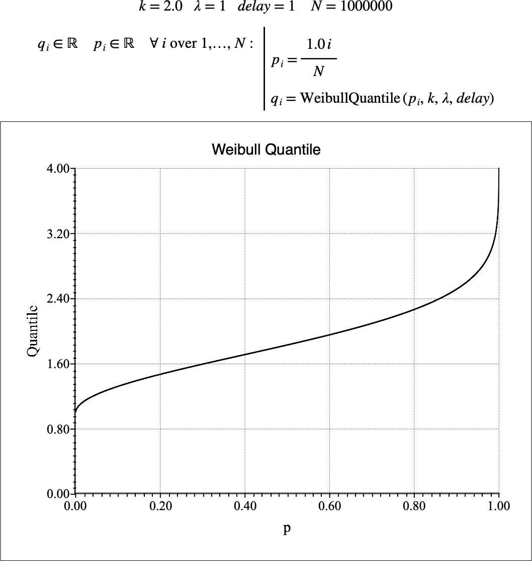
Figure 221 Example Use Of the WeibullQuantile Function