\(\text{BinomialCDF}\)
You can use the \(\text{BinomialCDF}\) function to calculate the cumulative distribution function (CDF) of the binomial distribution.
You can use the \binomialc backslash command to insert this function.
The following variants of this function are available:
\(\text{real } \text{BinomialCDF} \left ( \text{<k>}, \text{<n>}, \text{<p>} \right )\)
Where \(k\), \(n\), and \(p\) are scalar values. Note that this
function is defined over the range \(k \geq 0\), \(n \geq 0\), and
\(0 \leq p \leq 1\) and will either generate a run-time error or return
NaN for all other values.
The value is calculated directly from the incomplete regularized beta function by the relation:
Where \(\text{I} _ x\) represents the incomplete regularized beta function which is internally calculated using the Boost C++ library implementation.
The binomial distribution can be used to determine the probability of \(k\) successes in \(n\) trials of an experiment where each trial has an independent probability of success \(p\). The distribution also assumes that each trial does not result in the reduction of the size of the sample population.
Example applications of the binomial distribution may include.
Determining the probability of drawing \(k\) cards of a specific suit after \(n\) trials where cards are returned and the deck is shuffled after each trial.
Determining the approximate probability of grabbing \(k\) black marbles from a handful of \(n\) marbles after blindly reaching into large bin where black marbles make of \(p\) fraction of the total population.
Figure 109 shows the basic use of the \(\text{BinomialCDF}\) function.
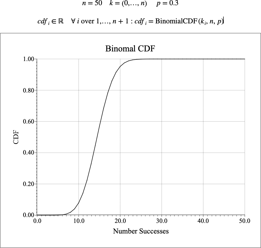
Figure 109 Example Use Of The BinomialCDF Function