\(\text{ExponentialQuantile}\)

You can use the \(\text{ExponentialQuantile}\) function to calculate the quantile function of the exponential distribution. The quantile function is the inverse of the cumulative distribution function.

You can use the \exponentialq backslash command to insert this function.

The following variants of this function are available:

• \(\text{real } \text{ExponentialQuantile} \left ( \text{<p>}, \text{<}\lambda\text{>} \right )\)

Where \(p\) and \(\lambda\) are scalar values representing the probability and the rate term respectively. Note that this function is defined over the range \(\lambda > 0\) and \(p \leq 0 \leq 1\) and will generate a runtime error or return NaN for values for which the function is not defined.

The value is calculated directly using the relation:

\[\text{ExponentialQuantile} \left ( p, \lambda \right ) = - \frac { \ln \left ( 1 - p \right ) } { \lambda }\]

The exponential distribution, along with the geometric distribution, has the property that the probability of an event occuring over some interval is independent of the start time of that interval.

\[Pr \left ( T \leq t _ 1 | T \geq t _ 0 \right ) = Pr \left ( 0 \leq T \leq t _ 1 - t _ 0 \right )\]

Where \(0 \leq t _ 0 \leq t _ 1\).

The exponential distribution is often used to model traffic from uncorrelated sources, such as arrival of cars at an intersection or customers into a queue. The exponential distribution is a special case of both the gamma distribution and the Erlang distribution.

The exponential distribution is also often used to model failure rate and is a special case of Weibull distribution.

Figure 132 shows the basic use of the \(\text{ExponentialQuantile}\) function.

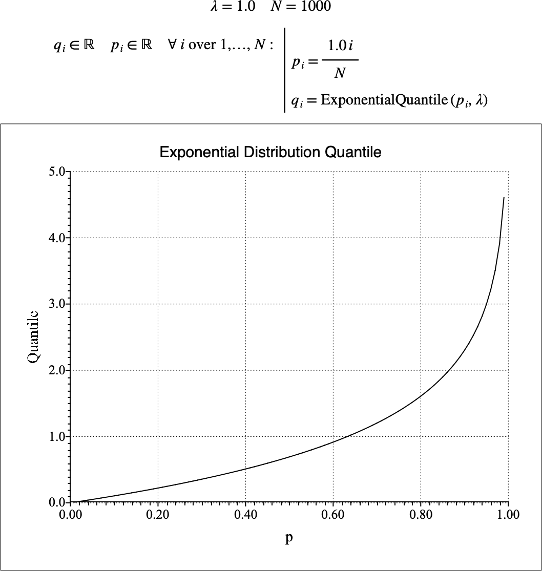
Figure 132 Example Use Of the ExponentialQuantile Function