\(\text{GeometricPMF}\)

You can use the \(\text{GeometricPMF}\) function to calculate the probability mass function (PMF) of the geometric distribution.

You can use the \geometricp backslash command to insert this function.

The following variants of this function are available:

• \(\text{real } \text{GeometricPDF} \left ( \text{<k>}, \text{<p>} \right )\)

Where \(k\) is a positive integer value representing the number of trials and \(p\) represents the success probability for each trial. Note that the \(\text{GeometricPMF}\) function is defined over the range \(k > 0\) and \(0 \leq p \leq 1\) and will generate a runtime error or return NaN for all other values.

The value is calculated directly using the relation:

\[\text{GeometricPMF} \left ( k, p \right ) = \left ( 1 - p \right ) ^ { k - 1 } p\]

The geometric distribution calculates the probability of success after \(k\) trials where the probability of success for any given trial is given by \(p\).

As an example, imagine you are drawing cards from an infinitely large shuffled deck. The probability of drawing a club for the first time when drawing the third card from the deck would be \(\text{GeometricPMF} \left ( 3, \frac{1}{4} \right )\)

Note that, like the exponential distribution, the geometric distribution models a memoryless process where the outcome from any trial is independent of the outcome of previous trials. The geometric distribution models discrete memoryless processes whereas the exponential distribution models continuous processes.

Figure 148 shows the basic use of the \(\text{GeometricPMF}\) function.

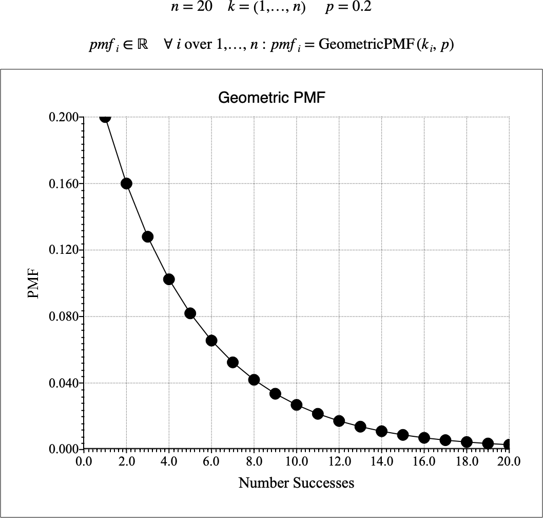
Figure 148 Example Use Of The GeometricPMF Function