\(\text{GeometricVariate}\)
You can use the \(\text{GeometricVariate}\) function to calculate one or more random variates in a geometric distribution.
You can use the \geometricv backslash command to insert this function.
The following variants of this function are available:
\(\text{integer } \text{GeometricVariate} \left ( \text{<p>} \right )\)
\(\text{integer matrix } \text{GeometricVariate} \left ( \text{<number rows>}, \text{<number columns>}, \text{<p>} \right )\)
Where \(p\) is a scalar values. Note that this function is defined over
the range \(0 \leq p \leq 1\) and will either generate a run-time error or
return NaN, or a matrix of NaN for all other input values.
The three parameter version, which includes \(\text{<number rows>}\) and \(\text{<number columns>}\) fields, returns an integer matrix returning random deviates. The single parameter version returns a single value.
This function calculate random variates using transformation method by:
Where \(u\) is a random variate over a uniform distribution over the range \(0 < u < 1\).
The geometric distribution calculates the probability of success after \(k\) trials where the probability of success for any given trial is given by \(p\).
As an example, imagine you are drawing cards from an infinitely large shuffled deck. The probability of drawing a club for the first time when drawing the third card from the deck would be \(\text{GeometricCDF} \left ( 3, \frac{1}{4} \right )\)
Note that, like the exponential distribution, the geometric distribution models a memoryless process where the outcome from any trial is independent of the outcome of previous trials. The geometric distribution models discrete memoryless processes whereas the exponential distribution models continuous processes.
Figure 147 shows the basic use of the \(\text{GeometricCDF}\) function.
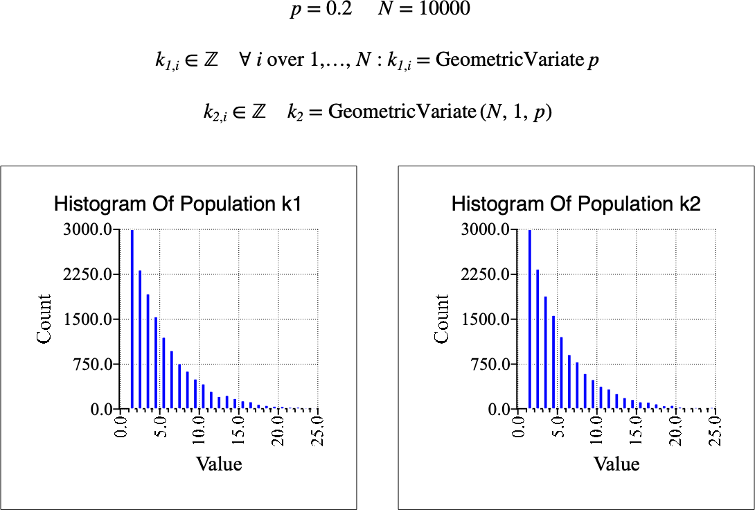
Figure 149 Example Use Of The GeometricVariate Function