\(\text{LogNormalPDF}\)

You can use the \(\text{LogNormalPDF}\) function to calculate the probability density function (PDF) of the log-normal distribution.

You can use the \lognormalp backslash command to insert this function.

The following variants of this function are available:

• \(\text{real } \text{LogNormalPDF} \left ( \text{<x>} \right )\)

• \(\text{real } \text{LogNormalPDF} \left ( \text{<x>}, \text{<}\mu\text{>} \right )\)

• \(\text{real } \text{LogNormalPDF} \left ( \text{<x>}, \text{<}\mu\text{>}, \text{<}\sigma\text{>} \right )\)

Where \(x\), \(\mu\), and \(\sigma\) are scalar values representing the value of interest, the mean value and the standard deviation. If not specified, the mean value will be 0 and the standard deviation will be 1. Note that this function is defined over the range \(x > 0\) and \(\sigma > 0\). The \(\text{LogNormalPDF}\) function will generate a runtime error or return NaN for values for which the function is not defined.

The value is calculated directly using the relation:

\[\text{LogNormalPDF} \left ( x, \mu, \sigma \right ) = \frac{1}{x \sigma \sqrt{2 \pi}} e ^ { - \frac{ \left [ \ln \left ( x \right ) - \mu \right ] ^ 2} {2 \sigma ^ 2} }\]

Figure 175 shows the basic use of the \(\text{LogNormalPDF}\) function.

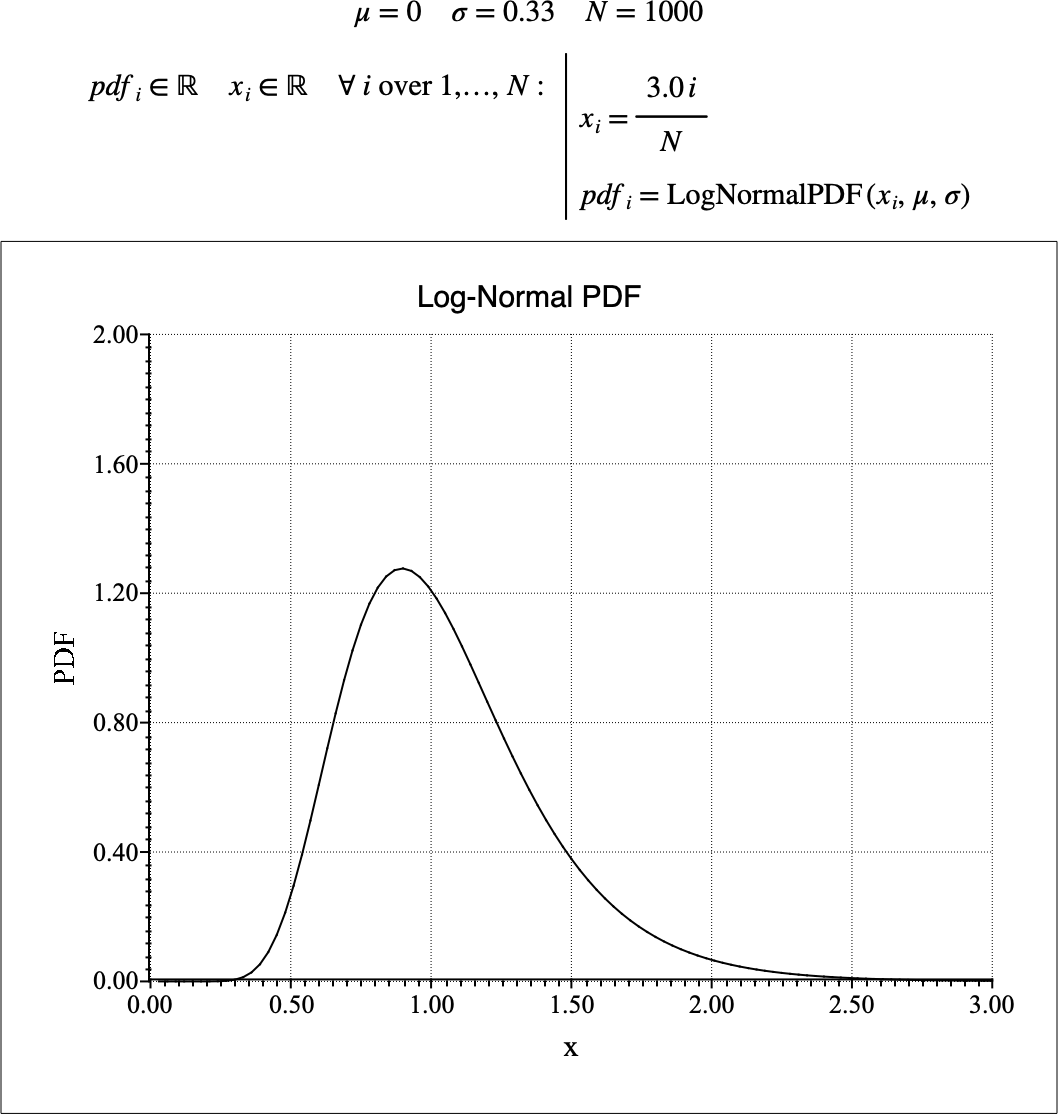
Figure 175 Example Use Of the LogNormalPDF Function