\(\text{LogNormalQuantile}\)

You can use the \(\text{LogNormalQuantile}\) function to calculate the quantile function of the log-normal distribution. The quantile function is the inverse of the cumulative distribution function.

You can use the \lognormalq backslash command to insert this function.

The following variants of this function are available:

• \(\text{real } \text{LogNormalQuantile} \left ( \text{<p>} \right )\)

• \(\text{real } \text{LogNormalQuantile} \left ( \text{<p>}, \text{<}\mu\text{>} \right )\)

• \(\text{real } \text{LogNormalQuantile} \left ( \text{<p>}, \text{<}\mu\text{>}, \text{<}\sigma\text{>} \right )\)

Where \(p\), \(\mu\), and \(\sigma\) are scalar values representing the probability, the mean value and the standard deviation. If not specified, the mean value will be 0 and the standard deviation will be 1. Note that this function is defined over the range \(0 \leq p \leq 1\) and \(\sigma > 0\). The \(\text{LogNormalQuantile}\) function will generate a runtime error or return NaN for values for which the function is not defined.

The value is calculated directly using the relation:

\[\text{LogNormalQuantile} \left ( p, \mu, \sigma \right ) = e ^ { \mu + \sqrt{2 \sigma ^ 2} \text{erf}^{-1} \left ( 2 p - 1 \right ) }\]

Where \(\text{erf}^{-1}\) represents the inverse error function.

Figure 176 shows the basic use of the \(\text{LogNormalQuantile}\) function.

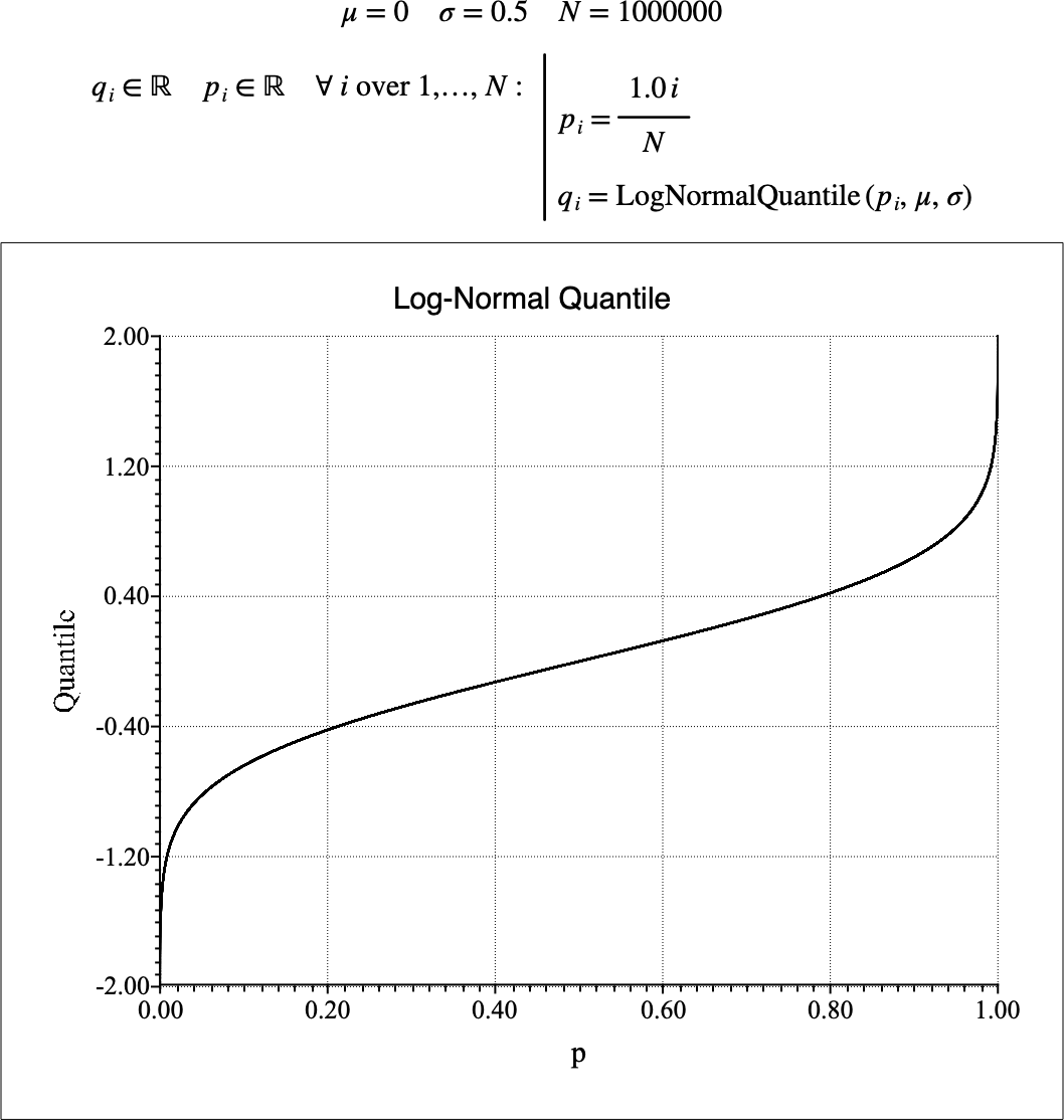
Figure 176 Example Use Of the LogNormalQuantile Function