Advanced Topics
This section discusses several more advanced aspects of Aion.
Algorithmic Complexity And Memory Usage
We often estimate the complexity of an algorithm based on the number of times the algorithm must repeat or iterate to complete a task. If an algorithm requires \(\alpha N\) iterations to perform a computation on data containing \(N\) members, where \(\alpha\) is approximately constant, then we say the complexity of the algorithm is \(\text{O} \left ( N \right )\). We refer to this notation as ‘’Big-O’’ notation for the complexity of the algorithm.
In addition, different complex data structures require memory which are allocated as needed as the data structures are modified.
Sets
Table 17 provides the average complexity for common set operations. Note that \(N\) represents the number of members in the set. When two sets are involved, \(N _ A\) represents the number of members for the first set and \(N _ B\) represents the number of members for the second set.
Operation |
Complexity |
|---|---|
Add a new member |
\(\text{O} \left ( \log N \right )\) |
Remove a member |
Between \(\text{O} \left ( 1 \right )\) and \(\text{O} \left ( \log N \right )\) |
\(a \in S\) |
\(\text{O} \left ( 1 \right )\) |
\(A \cup B\) |
\(\text{O} \left [ \min \left ( N _ A, N _ B \right ) \log \left ( \max \left ( N _ A, N _ B \right ) \right ) \right ]\) |
\(A \cap B\) |
\(\text{O} \left [ \min \left ( N _ A , N _ B \right ) \right ]\) |
\(A \sqcup B\) |
\(\text{O} \left [ \log \left ( N _ A + N _ B \right ) \right ]\) |
\(A \times B\) |
\(\text{O} \left [ \log \left ( N _ A N _ B \right ) \right ]\) |
\(\text{Sort } A\) |
Approximately \(\text{O} \left ( N \right )\) |
Aion sets allocate memory in blocks as the number of set members increases, typically each new reservation roughly doubles the number of allocated members, adjusted slightly to enforce rules required by the Aion set algorithm. For sets containing simple data types, the allocated blocks provide all the storage that is needed for the set. Also note that Aion sets will always maintain some unused space in order to limit the statistical probability of collisions during hash table lookups.
Tuples
Table 18 provides the average complexity for common operations on tuples. Note that \(N\) represents the number of members in the tuple. When two sets are involved, \(N _ A\) represents the number of members for the first tuple and \(N _ B\) represents the number of members for the second set.
Operation |
Complexity |
|---|---|
Append an element |
\(\text{O} \left ( \log 1 \right )\) |
Prepend an element |
\(\text{O} \left ( N \right )\) |
Remove a member |
\(\text{O} \left ( N \right )\) |
\(A _ i\) |
\(\text{O} \left ( 1 \right )\) |
\(A _ { a, \ldots, b }\) |
\(\text{O} \left ( \left | b - a \right | \right )\) |
\(A \cdot B\) |
\(\text{O} \left ( N _ A + N _ B \right )\) |
\(\text{Alph } A\) |
\(\text{O} \left ( N \log N \right )\) |
\(\text{Sort } A\) |
\(\text{O} \left ( N \log N \right )\) |
Tuples currently allocate memory in blocks, doubling the size of the blocks each time the tuple needs to grow.
Boolean Matrices
Table 19 provides the average complexity for common operations on boolean matrices. Note that \(N\) represents the number of coefficients in the matrix, \(N _ r\) represents the number of matrix rows, and \(N _ c\) represents the number of matrix columns. When two matrices are involved, each term will be postpended with \(a\) or \(b\) respectively.
Operation |
Complexity |
|---|---|
\(\begin{bmatrix} A & 2 \\ b & 3 \end{bmatrix}\) |
\(\text{O} \left ( N \right )\) |
\(A _ i\) or \(A _ { i,j }\) where \(i \leq N _ r \land j \leq N _ c\) |
\(\text{O} \left ( 1 \right )\) |
\(A _ i\) or \(A _ { i,j }\) where \(i > N _ r \lor j > N _ c\) |
Approximately \(\text{O} \left ( \max \left ( N_r, i \right ) \max \left ( N _ c, j \right ) \right )\) |
\(A _ { a, \ldots, b }\) |
\(\text{O} \left ( \left | b - a \right | \right )\) |
\(A _ { \left ( a, \ldots, b \right ), \left ( c, \ldots, d \right ) }\) |
\(\text{O} \left ( \left | b - a \right | \left | d - c \right | \right )\) |
\(\left [ A | B \right ]\) |
\(\text{O} \left [ \max \left ( N _ { ra }, N _ { rb } \right) \left ( N _ { ca } + N _ { cb } \right ) \right ]\) |
\(\left [ \frac{A}{B} \right ]\) |
\(\text{O} \left ( \left ( N _ { ra } + N _ { rb } \right) \max \left ( N _ { ca }, N _ { cb } \right ) \right )\) |
\(A ^ T\) |
\(\text{O} \left ( 1 \right )\) |
Boolean matrices currently store data in bit packed format, one bit per coefficient. For the matrix below:
The matrix would be packed in memory as shown in Figure 103. Data is packed with one bit per coefficient by column, then by row. Columns are padded such that the length is a power of 2 number of bits up-to 512 columns. For matrices with more than 512 columns, columns will be padded to a multiple of 512 columns.
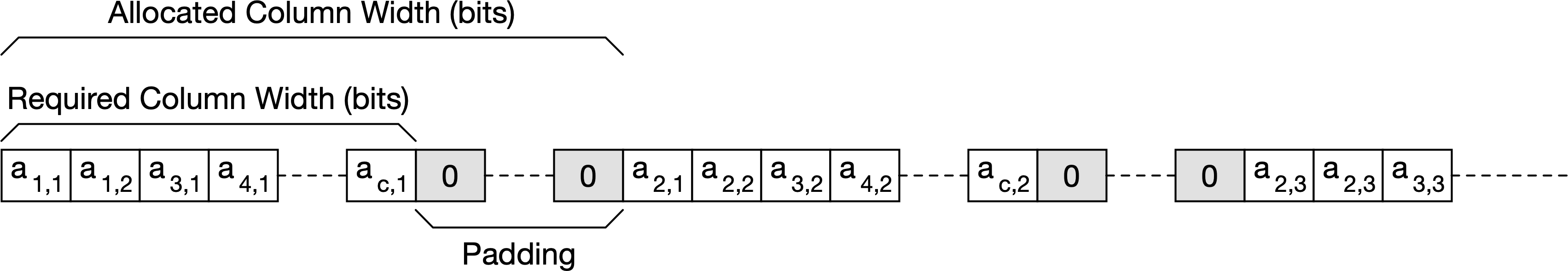
Figure 103 Boolean Matrix Memory Structure
For example:
A matrix with 1 row and 120 columns would allocate 128 bits for the column and would allocate a total of 16 bytes for the entire matrix.
A matrix with 90 rows and 1 column would allocate 1 bit for each column and would allocate a total of 90 bits or 12 bytes for the entire matrix.
A matrix with 10 rows and 13 columns would allocate 16 bits to each column and would allocate a total of 160 bits or 20 bytes for the entire matrix.
A matrix with 500 rows and 1300 columns would allocate 1536 bits to each column and would allocate a total of 768,000 bits or 96,000 bytes for the entire matrix.
When the number of columns in a matrix changes, the matrix will use the remaining padding, if possible. If the new size requires more column padding than is available, Aion will allocate new memory for the matrix and repack the data using the rules described above. In a few cases, Aion can also avoid allocating memory by repacking data in-place.
Integer, Real, And Complex Matrices
Table 20 provides the average complexity for common operations on integer, real, and complex matrices. Note that \(N\) represents the number of coefficients in the matrix, \(N _ r\) represents the number of matrix rows, and \(N _ c\) represents the number of matrix columns. When two matrices are involved, each term will be postpended with \(a\) or \(b\) respectively.
Operation |
Complexity |
|---|---|
\(\begin{bmatrix} A & 2 \\ b & 3 \end{bmatrix}\) |
\(\text{O} \left ( N \right )\) |
\(A _ i\) or \(A _ { i,j }\) where \(i \leq N _ r \land j \leq N _ c\) |
\(\text{O} \left ( 1 \right )\) |
\(A _ i\) or \(A _ { i,j }\) where \(i > N _ r \lor j > N _ c\) |
Approximately \(\text{O} \left ( \max \left ( N_r, i \right ) \max \left ( N _ c, j \right ) \right )\) |
\(A _ { a, \ldots, b }\) |
\(\text{O} \left ( \left | b - a \right | \right )\) |
\(A _ { \left ( a, \ldots, b \right ), \left ( c, \ldots, d \right ) }\) |
\(\text{O} \left ( \left | b - a \right | \left | d - c \right | \right )\) |
\(\left [ A | B \right ]\) |
\(\text{O} \left [ \max \left ( N _ { ra }, N _ { rb } \right) \left ( N _ { ca } + N _ { cb } \right ) \right ]\) |
\(\left [ \frac{A}{B} \right ]\) |
\(\text{O} \left ( \left ( N _ { ra } + N _ { rb } \right) \max \left ( N _ { ca }, N _ { cb } \right ) \right )\) |
\(A ^ T\), \(A ^ {*}\), \(A ^ H\) |
\(\text{O} \left ( 1 \right )\) |
\(A + B\), \(A - B\) |
\(\text{O} \left ( N \right )\) |
\(A B\) |
\(\text{O} \left ( N ^ 3 \right )\) |
\(A \circ B\) |
\(\text{O} \left ( N \right )\) |
\(A \otimes B\) |
\(\text{O} \left ( N _ a N _ b \right )\) |
Integer, real, and complex matrices currently store data in dense column major format. Row matrices include no padding between columns. In all other cases, space for columns are allocated in multiples of 64 bytes to optimize for the use of SIMD instructions. Table 21 lists the padding in terms of coefficients for different types of matrices.
Matrix Type |
Columns Allocated In Multiples Of |
|---|---|
Integer Matrices |
8 Coefficients |
Real Matrices |
8 Coefficients |
Complex Matrices |
4 Coefficients |
When the number of columns in a matrix changes, the matrix will use the remaining padding, if possible. If the new size requires more column padding than is available, Aion will allocate new memory for the matrix and repack the data using the rules described above. In a few cases, Aion can also avoid allocating memory by repacking data in-place.
Note
Future versions of Aion may support multiple matrix structures such as triangular matrices and sparse matrices. Those matrices will maintain data using structures different from those described here.
Optimizations
Aion will perform a number of optimizations to improve the performance of algorithms and models. Knowledge of how these optimizations work can help you gain the most benefit from Aion.
Note that this section only discusses a subset of the optimizations that are performed. In addition to high level operations, Aion uses the LLVM backend to generate executable code and leverages many of the optimizations available through LLVM.
Use Of Multiple Cores
Aion will distribute some very time intensive calculates across multiple processor cores. This capability is currently limited to certain real and complex matrix operations.
Use Of SIMD Instuctions
Where appropriate, Aion will make use of processor SIMD instructions to parallelize operations performed on large collections of data. This capability is currently limited to real and complex matrix operations.
Memoization
Memoization is a common optimization technique used to optimize functions that tend to be called with the same parameter values or tend to require the same intermediate values.
For example, to calculate \(n!\), we need to calculate \(\left (n - 1 \right ) !\) first. Once Aion calculates the factorial of a value, it stores the result and all intermediate results for future reference. The factorial operator only needs to perform calculations if it has not already calculated the result for a given value.
Other functions, such as many of the functions used to calculate random variates, must calculate multiple intermediate values for the distribution using the supplied distribution parameters. Since these functions tend to be called with the same distribution parameters, they store off as many intermediate values as possible and only calculate new intermediate values if the distribution parameters change.
Copy On Write
Copy-on-write is a common optimization technique used to both reduce memory usage and to improve performance. The technique is used extensively with the following types of data:
Sets
Tuples
Matrices
Each of these data structures maintains a reference count of the number of variables that reference the data. When you create a complex structure such as a matrix:
Aion allocates memory for the matrix, populates the memory with the values and assigns a reference count of 1 to the allocated memory.
If we modify \(A\) using an expression such as:
Aion will check the reference count, see that only one variable references the data and modify existing matrix contents, in-place.
When we assign a new variable to \(A\), say with the statement:
The variable \(B\) will in fact reference the exact same data as \(A\). The reference count tied to the data will be incremented from 1 to 2 to indicate that two variables reference the data. The assignment completes very quickly because no data is copied and only a single location, the reference count, is changed.
If we then perform an operation such as:
Aion will look at the reference count, determine that two variables reference the data and only then then make an actual copy of the data. The new copy is assigned a reference count of 1 since it’s a new copy of the data. The reference count on the original data is also reduced by 1 because there is one fewer reference to that data.
Lazy Evaluation
Lazy evaluation is a technique used with matrices to reduce the total processing overhead.
Lazy evaluation delays a number of memory intensive operation until they can be performed in combination, reducing the total memory bandwidth required.
The following matrix operations are evaluated lazily:
\(A ^ T\)
\(A ^ {*}\)
\(A ^ H\)
\(\alpha A\) where \(\alpha\) is a basic type.
\(\frac{A}{\alpha}\) where \(\alpha\) is a basic type.
When any of these operations are performed, the matrix stores side-band information indicating that a transpose, conjugate, or conjugate transpose needs to be performed and/or adjusts basic scale terms carried with the matrix.
The net effect is that matrix transpose, conjugate, conjugate transpose and operations against basic types will be performed on matrices extremely quickly.
The operations above are evaluated when an operation is encountered on a matrix that requires traversal of the entire matrix. Several operations, such as querying the value of individual coefficients may also trigger evaluation of lazy operations.
Note that lazy evaluation is managed independently from copy-on-write. Data will be shared between matrices even after performing any of the lazy operations listed above since the raw data does not need to be changed.
Optimizations Of The Forall Operator
Normally if you create expressions such as
Aion must create the set X then iterate the set for each value. While Aion attempts to do this as efficiently as possible, doing so would normally be less efficient than a construct such as:
If you define the set containing a range or define a range directly in the \(\forall\), Aion will optimize the \(\forall\) operator to yield similar efficiencies.
Constructs such as:
Will all yield similar efficiencies as the while loop shown above.
Optimized Use Of Functions And Operators
Aion can sometimes optimize the use of functions and operators to improve accuracy and performance. Currently there are only a limited number of cases where Aion will perform these optimizations.
As an example, Aion will identify constructs such as \(\log _ b \left ( \Gamma x \right )\) and will directly calculate the log-gamma function rather than calculate \(\Gamma x\) then take the \(\log _ b\) of the result.
Similar optimizations exist for other combinations of functions and operators.
Combining functions and operators will improve accuracy and performance of your algorithms and models and should be transparent. If absolutely necessary, you can force the operations to be performed independently by either:
Using an intermediate variable to temporarily hold the intermediate result.
Use the parenthesis, bracket, or brace grouping operator found on the Basic Math Dock to logically separate the operations. Note that simply adding parenthesis, brackets, or braces using the Operator Format Dialog or Operator Dock will not disable these optimizations.
Inesonic, LLC will continue to expand the optimizations that are performed as Aion evolves.